Bellman Equation in Reinforcement Learning

Image Credits

Introduction: The Heartbeat of Every RL Algorithm

If reinforcement learning has a single soul, it is the Bellman equation. Every algorithm you have ever heard of — Q-learning, DQN, PPO, RLHF — is either solving it, approximating it, or bootstrapping from it. Understanding the Bellman equation is not merely an academic exercise; it is the gateway to understanding why reinforcement learning works at all.

At its core, the Bellman equation captures one profoundly simple insight: the value of being somewhere now equals the immediate reward you receive, plus the discounted value of wherever you end up next. That recursive observation, formalized by the American mathematician Richard Ernest Bellman in the early 1950s, transformed decision-making theory and quietly became the mathematical backbone of modern artificial intelligence.

1. Historical Context: Who Was Richard Bellman?

Richard Ernest Bellman was born in Brooklyn, New York, on August 26, 1920. A prodigy who topped all New York school pupils in mathematics in his final year, he went on to Princeton for his PhD and later joined the RAND Corporation, where he developed the ideas that would shape an entire field.

Bellman introduced the concept of dynamic programming in 1953 — a method for solving complex sequential decision-making problems by breaking them into simpler, overlapping subproblems. The term "dynamic" was chosen deliberately: Bellman later admitted it was partly chosen because it sounded impressive enough that even government officials would not object to funding it.

The equation that carries his name first appeared in that context. Over his career,

Bellman received:

• The John von Neumann Theory Prize (1976) from the Operations Research Society of America

• The IEEE Medal of Honor (1979), for contributions to decision processes and control theory

• Election to the National Academy of Sciences (1983)

• The posthumously established Richard E. Bellman Control Heritage Award, the highest honor in the American control systems community

His work laid the mathematical foundation not just for dynamic programming, but for the entire modern field of reinforcement learning.

2. The Reinforcement Learning Setup: The Stage the Bellman Equation Plays On

Before the equation itself, we need to understand the environment in which it operates. Reinforcement learning models the interaction between an agent and an environment as a Markov Decision Process (MDP).

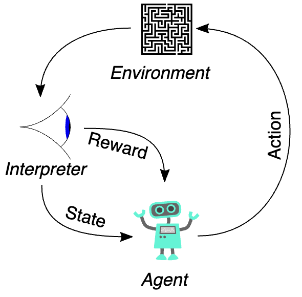
The agent-environment loop: the agent observes state sₜ, takes action aₜ, receives reward rₜ₊₁, and transitions to state sₜ₊₁. Source: Wikimedia Commons

The MDP Components

An MDP is formally defined as the tuple (S, A, T, R, γ), where each component carries a precise meaning:

• S — The state space: the complete set of situations the agent can find itself in. This could be a chess board position, the pixels of an Atari game screen, or the joint angles of a robotic arm.

• A — The action space: every move available to the agent at any given state. Actions can be discrete (left, right, up, down) or continuous (apply 3.2 Nm of torque).

• T(s′ | s, a) — The transition function: the probability of landing in state s′ after taking action a in state s. This encodes the stochastic dynamics of the environment.

• R(s, a, s′) — The reward function: the scalar signal the agent receives after transitioning. It is the only feedback mechanism — the teacher whose grades the agent spends its entire existence trying to improve.

• γ ∈ [0, 1) — The discount factor: a number that controls how much the agent cares about the future versus the present.

The Markov Property

The "Markov" in MDP comes from a crucial assumption: the future depends only on the current state, not on the history of how you got there.

This is not just a mathematical convenience — it is what makes the problem tractable. Without it, the agent would need to remember its entire history of interactions to make any decision. With it, the current state is a sufficient statistic for everything that matters.

3. Return and Discounting: What the Agent Is Trying to Maximize

The agent does not try to maximize the next reward. It tries to maximize the total cumulative discounted return from the current timestep onwards:

This formulation raises an immediate question: why discount? The discount factor γ serves several essential purposes:

• Mathematical convergence — Without γ < 1, the sum G_t could diverge to infinity for continuing (non-terminating) tasks.

• Economic intuition — A reward received now is more certain and more valuable than a reward promised in the distant future. This mirrors human temporal preferences.

• Computational stability — Smaller γ makes the agent focus on near-term consequences, which can make learning faster but more myopic. Larger γ encourages long-horizon planning but can slow convergence.

The effect of different γ values on agent behavior:

4. Policy and Value Functions: The Two Things an Agent Learns

Every RL agent is, at its core, learning one or both of two things.

The Policy π

A policy π maps states to actions (or distributions over actions). It is the agent's complete strategy — given any state it could find itself in, the policy tells it what to do. Formally:

• Deterministic policy: π(s) = a — always take action a in state s

• Stochastic policy: π(a|s) = P(A=a | S=s) — sample from a distribution over actions given state s

The goal of RL is to find the optimal policy π* — the strategy that maximizes expected return from every state.

The Value Function V^π(s)

The state-value function measures how good it is to be in state s, given that the agent follows policy π from that point forward:

Every policy induces a different value function. A bad policy produces low V everywhere. An optimal policy produces the highest achievable V — this is called V*(s).

The Action-Value Function Q^π(s, a)

The action-value function (also called the Q-function) measures how good it is to take action a from state s, and then follow policy π thereafter:

The Q-function is arguably more important in practice than V, because it contains the information needed to act — you choose the action with the highest Q-value in your current state.

5. The Bellman Equation: Four Forms

Now we arrive at the equation itself. The Bellman equation expresses V and Q recursively — in terms of themselves at the next timestep. This is the bootstrapping insight that makes everything tractable.

The Bellman backup: from state s, consider all actions under policy π, all possible next states s′ under transition T, then fold the future value back to the present. Source: GeeksforGeeks

Form 1: Bellman Expectation Equation for V^π

Reading this equation piece by piece:

• π(a|s) — how likely is the agent to choose action a under its current policy?

• T(s′|s,a) — if it takes action a, how likely is it to land in s′?

• R(s,a,s′) — what reward does it receive for this transition?

• γ · V^π(s′) — what is the discounted value of being in s′ and following π from there?

The double sum averages over both the stochasticity of the policy and the stochasticity of the environment. The result is a self-consistent recursive equation — solve it and you have the true value of every state under π.

Form 2: Bellman Expectation Equation for Q^π

This is the Q-function analog. Note how Σ_{a'} π(a'|s') · Q^π(s',a') is exactly V^π(s′) — confirming the relationship between V and Q. The two forms are equivalent; they are just written with different quantities on the left-hand side.

The bridge between V and Q in both directions:

Form 3: Bellman Optimality Equation for V*

The expectation equations evaluate a fixed policy. The optimality equations ask: what is the best possible value, across all policies?

The critical difference from Form 1: the sum over π(a|s) is replaced by a max over actions. We no longer ask what π would do — we ask what the best possible action is. This nonlinearity (the max operator) means the optimality equation cannot be solved with linear algebra and requires iterative methods.

Once V* is known, the optimal policy is trivially:

Form 4: Bellman Optimality Equation for Q*

This is the most important form for model-free reinforcement learning. The max_{a'} Q*(s', a') term says: from the next state, assume we will take the single best possible action. This makes Q-learning off-policy — it always bootstraps from the optimal next action, regardless of what the agent actually did.

Once Q* is known, the optimal policy is even simpler — just pick the greedy action at every state:

6. The Contraction Mapping Theorem: Why Bellman Converges

A natural question: how do we know iteratively applying the Bellman equation converges to the right answer? The answer lies in a fundamental result from functional analysis.

Define the Bellman operator T* as the operation of applying the right-hand side of the optimality equation once:

The Bellman operator is a γ-contraction in the sup-norm: for any two value functions V and U,

Since γ < 1, every application of T* brings estimates closer together by a factor of γ. By the Banach fixed-point theorem, this contraction has a unique fixed point — and that fixed point is exactly V*. Starting from any initial guess V₀, repeated application of T* converges:

This is the theoretical guarantee behind value iteration, and it explains why Bellman-based algorithms provably converge.

7. From Theory to Algorithm: How the Bellman Equation Drives RL Methods

The Bellman equation is not just mathematics — it is an algorithm blueprint. Different RL algorithms can be understood as different strategies for solving or approximating the

The full family of RL algorithms — from dynamic programming to deep RL — all flow from the Bellman equation.

7.1 Dynamic Programming: Solving Bellman Exactly

When the full model (T and R) is known, the Bellman equation can be solved exactly through dynamic programming methods.

Value Iteration applies the Bellman optimality operator repeatedly until convergence:

Each sweep over all states brings the estimate closer to V*. The algorithm terminates when the maximum change across all states falls below a threshold ε.

Policy Iteration alternates between two phases:

• Policy Evaluation: given the current policy π_k, solve the Bellman expectation equation to find V^{π_k} exactly (via linear algebra or iterative updates)

• Policy Improvement: extract a better policy by acting greedily with respect to V^{π_k}

Policy iteration often converges in fewer iterations than value iteration because the policy improvement step exploits the structure of the problem more efficiently.

Key properties of dynamic programming:

• Requires a complete model of the environment (T and R)

• Guarantees convergence to the globally optimal policy

• Computationally expensive for large state spaces (the "curse of dimensionality")

• Mostly used as a theoretical benchmark rather than a practical algorithm

7.2 Temporal Difference Learning: Bootstrapping Without a Model

In most real-world problems, the transition function T and reward function R are unknown. The agent must learn from experience — observing transitions (s, a, r, s′) and using them to estimate V or Q.

Temporal Difference (TD) learning is the key idea: instead of waiting until the end of an episode to compute the true return, use the Bellman equation as an update target after each single step:

The TD error δ_t is the gap between what the agent expected (V(s_t)) and what the Bellman equation says it should expect (r_t + γV(s_{t+1})). This error is propagated backward, slowly correcting estimates toward their Bellman-consistent values.

Key properties of TD learning:

• Model-free — no knowledge of T or R required

• Online — updates after every single step, not at the end of an episode

• Bootstraps — uses its own estimate V(s_{t+1}) as the target (unlike Monte Carlo which waits for the true return)

• The TD error δ_t is directly related to dopamine signals in neuroscience — an early finding that suggests RL captures something fundamental about biological learning

7.3 Q-Learning: The Bellman Optimality Equation as an Update Rule

Q-learning is perhaps the most direct algorithmic expression of the Bellman optimality equation. Given a sampled transition (s, a, r, s′), the Q-learning update is:

Reading this carefully:

• r + γ · max_{a'} Q(s′, a′) is the Bellman optimality target — what Q(s,a) should be according to the equation

• Q(s,a) is the current (incorrect) estimate

• The difference is the error, and α controls how aggressively we correct it

Because Q-learning always bootstraps from max_{a'} Q(s′, a′) regardless of which action was actually taken, it is off-policy — it can learn the optimal Q-function even while following an exploratory (non-optimal) behavior policy like ε-greedy.

SARSA, by contrast, is on-policy: it uses the Q-value of the action actually taken next:

where a′ is the action the policy actually selected at s′. This makes SARSA more conservative — it learns the value of the policy being followed, including its exploratory behavior.

8. Deep Q-Networks: The Bellman Equation at Scale

The classical Q-learning algorithm maintains a lookup table of Q-values indexed by (s, a) pairs. This works for small, discrete state spaces — but fails catastrophically for the real world. A single frame of an Atari game has approximately 256^(84×84×4) ≈ 10^{170,000} possible states. No table can hold that.

The breakthrough insight of Deep Q-Networks (DQN), introduced by DeepMind in 2015,

was to replace the table with a neural network that approximates the Q-function:

where θ are the neural network weights trained by gradient descent. The loss function is derived directly from the Bellman equation:

DQN uses a convolutional neural network to map raw game pixels directly to Q-values for each possible action — a direct instantiation of the Bellman optimality equation at scale. Source: ResearchGate

DQN introduced two crucial stabilization tricks to prevent the Bellman bootstrap from diverging:

Experience Replay:

• Instead of learning from consecutive transitions (which are highly correlated), store all transitions in a replay buffer D

• Sample random minibatches from D for each update

• Breaks correlation between consecutive samples, reduces variance, allows reusing past experience multiple times

Target Network:

• The Bellman target r + γ · max_{a'} Q(s′, a′; θ⁻) uses a separate, frozen network θ⁻

• θ⁻ is updated to match θ only every N steps (e.g., every 1000 steps)

• Prevents the target from moving with every update, stabilizing the optimization landscape

With these two modifications, DQN achieved superhuman performance on 49 Atari games from raw pixels — a landmark result that ignited modern deep reinforcement learning.

9. The Advantage Function: Bellman's Child

From the Bellman equations, a third fundamental quantity emerges naturally — the advantage function:

The advantage answers a more refined question: not "how good is action a?" (Q), nor "how good is this state?" (V), but "how much better is action a compared to what my policy would normally do in this state?"

• A > 0: action a is better than the policy's average choice — increase its probability

• A = 0: action a is exactly what the policy would do — no change needed

• A < 0: action a is worse than average — decrease its probability

The advantage function is lower variance than raw Q-values because V(s) acts as a baseline — it removes the component of Q that is due to being in a good or bad state (which is not under the agent's control at that moment) and isolates the component due to the specific action choice.

The advantage is central to modern actor-critic algorithms:

• A2C/A3C (Advantage Actor-Critic): uses A as the training signal for the policy gradient

• PPO (Proximal Policy Optimization): clips the policy update using A, preventing destructively large steps

• RLHF (Reinforcement Learning from Human Feedback): trains LLMs using PPO with A computed from a learned reward model

10. The Bellman Equation in Modern AI: RLHF and LLM Training

The Bellman equation did not stay confined to games and robots. In 2022–2026, it became the hidden engine inside large language model training.

RLHF (Reinforcement Learning from Human Feedback) — the technique used to fine-tune GPT, Claude, Gemini, and virtually every frontier language model — is an application of the Bellman equation at industrial scale:

1. A reward model R_θ is trained on human preference data to predict which responses humans prefer

2. The language model serves as the policy π_φ, mapping prompts (states) to tokens (actions)

3. PPO, which relies on the Bellman expectation equation to estimate advantages, is used to update π_φ to maximize R_θ while staying close to the original model

Every token generated by a modern LLM is, in a very real sense, an action in an MDP — and the Bellman equation is quietly computing how good that action was.

More recently, process reward models (PRMs) give step-level Bellman signals during reasoning — not just outcome-level feedback. This allows the model to receive credit (or blame) for each reasoning step, not just the final answer, dramatically improving mathematical and logical reasoning abilities.

11. Common Failure Modes: When Bellman Breaks Down

Understanding the Bellman equation also means understanding where it can fail in practice.

Bootstrapping instability: When using a neural network approximator, bootstrapping (using your own estimates as targets) can create a feedback loop. If Q(s′, a′; θ) is overestimated, the Bellman target becomes overestimated, which trains Q(s, a; θ) to be overestimated, which inflates targets for states that transition to s — a spiral of overestimation. Double DQN addresses this by using the main network to select actions and the target network to evaluate them.

Function approximation error: The contraction mapping guarantee assumes exact Bellman updates. With neural network approximation, each update introduces error. The projected Bellman error can accumulate, and in severe cases the value function diverges entirely — the "deadly triad" of function approximation + bootstrapping + off-policy learning.

Reward hacking: The Bellman equation maximizes whatever R(s,a,s′) specifies. If the reward function is misspecified, the agent will find and exploit the gap between what R measures and what you actually want — a phenomenon that afflicts RL systems from game-playing agents to RLHF-trained language models.

Sparse rewards and credit assignment: When rewards are rare (e.g., only at the end of a long episode), the Bellman target r + γV(s′) is dominated by γV(s′) for almost all transitions. The reward signal bleeds backward through the chain very slowly, making learning extremely sample-inefficient.

12. The Bellman Equation Across All RL Algorithms

13. Worked Example: Bellman in a 3-State Chain

To make the mathematics concrete, consider a simple 3-state chain: S₁ → S₂ → S₃ (goal). Actions are deterministic. Rewards: r = 0 for all transitions except reaching S₃, which gives r = +1. Discount γ = 0.9.

The Bellman expectation equations for a policy that always moves right:

Wait — S₃ is a terminal state, so V(S₃) = 1 (the final reward, no further discounting beyond it). Working backwards:

These values make intuitive sense: being in S₁ is worth 0.81 because the reward is 2 steps away and discounted by γ² = 0.81. Being in S₂ is worth 0.9 because the reward is 1 step away and discounted by γ¹ = 0.9. This is exactly what the TD learning simulation we described earlier converges to over many updates.

14. Key Takeaways

The Bellman equation is not one equation — it is a family of recursive relationships that tie together the past, present, and future of an RL agent's experience:

• It converts an infinite-horizon optimization problem into a tractable fixed-point problem, solvable by repeated iteration.

• It is the source of the bootstrapping idea — using current estimates to improve current estimates — that makes sample-efficient RL possible.

• Every major RL algorithm is a different strategy for solving or approximating one of the Bellman equation's four forms.

• The contraction mapping theorem guarantees that iterating the Bellman operator converges to the unique optimal value function V*.

• The advantage function A = Q − V, derived from the Bellman equations, is the central quantity in modern actor-critic algorithms including PPO and RLHF.

• In 2025–2026, the Bellman equation runs quietly inside every major AI system — from game-playing agents to language models trained with RLHF — making it not just historically important but actively central to the state of the art.

Richard Bellman described the principle behind his equation with characteristic simplicity: "An optimal policy has the property that whatever the initial state and initial decision are, the remaining decisions must constitute an optimal policy with regard to the state resulting from the first decision."

That is the principle of optimality. That is the Bellman equation. And that — recursively, relentlessly, one step at a time — is how machines learn to be intelligent.

References and Further Reading

• Sutton, R.S. & Barto, A.G. (2018). Reinforcement Learning: An Introduction (2nd ed.). MIT Press. [Free at incompleteideas.net]

• Bellman, R. (1957). Dynamic Programming. Princeton University Press.

• Mnih, V. et al. (2015). Human-level control through deep reinforcement learning. Nature, 518, 529–533.

• Schulman, J. et al. (2017). Proximal Policy Optimization Algorithms. arXiv:1707.06347.

• Dreyfus, S. (2002). Richard Bellman on the Birth of Dynamic Programming. Operations Research, 50(1), 48–51.

• Ouyang, L. et al. (2022). Training language models to follow instructions with human feedback. NeurIPS 2022.