


Proximal Policy Optimization(PPO)

Proximal Policy Optimization (PPO) was introduced in 2017 for simulated robots and Atari games, it became the optimization engine behind reinforcement learning from human feedback (RLHF) for large language models.

Introduction: One Algorithm, Two Worlds
Picture a legged robot learning to cross uneven ground. Each footstep changes what it will feel next, and a step that looks safe now can tip it over three steps later. Now picture a language model answering a question. Each token it writes changes the context for the next one, and a phrase that looks fluent now can lead the answer somewhere unhelpful or untrue.
These two problems look unrelated, yet they share a structure. In both, an agent makes a sequence of decisions, each decision shapes the situation that follows, and the verdict on the whole sequence arrives late. Reinforcement learning (RL) is the discipline built for exactly this setting: it optimizes a policy from interaction rather than fitting fixed input–target pairs.
Policy-gradient methods adjust that policy directly. Their weakness is noise. A small batch can make one action look unusually good, and an eager update can then change behavior too much. The robot falls; the language model learns to flatter a reward model instead of helping the user. PPO, introduced by Schulman and colleagues in 2017 [1], was designed to tame this: it lets a learner reuse fresh trajectories for several gradient steps while removing the objective's reward for extreme changes on any one sample.
That design is why PPO crossed over. When OpenAI's InstructGPT work set out to align a language model with human preferences, it treated generation as an RL problem and used PPO to optimize it [4]. The prompt and the text written so far became the state. Each token became an action. A reward model trained on human comparisons supplied the reward. The same clipped objective that steadies a walking robot now steadies a model with billions of parameters.
The central idea. Improve the current policy, but limit the optimization incentive to change any sampled action's probability by too much. PPO-Clip does this by clipping a probability ratio inside a surrogate objective. The ratio itself is not hard-constrained, and clipping alone does not prove that the policy stays within a fixed distance of its predecessor. Practical implementations therefore also watch approximate KL divergence and stop early when the policy moves more than intended.
Mathematical foundations
The Markov decision process
An RL task is usually modeled as a Markov decision process (MDP):
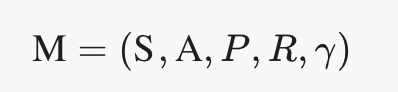
Here 𝓢 is the state space, 𝓐 the action space, P(s′ | s, a) the transition distribution, R(s, a) the reward function, and γ ∈ [0, 1) the discount on future rewards. At step t the agent observes sₜ, samples aₜ from its policy πθ, receives reward rₜ and moves to sₜ₊₁. For a robot, sₜ may hold joint angles and velocities; for a game agent, a screen image or a compact game state.

Return and objective
The discounted return from step t sums present and future rewards:

The policy objective is the expected return over trajectories the policy generates:

The policy decides which actions are taken, which states are visited and which rewards are seen. PPO raises J(θ) with policy-gradient estimates while moderating how much any one sample can reward a change in action probability.
Stochastic policies
A policy maps a state to a distribution over actions, πθ(a | s). With discrete actions, a network returns categorical probabilities. In continuous control, it returns the parameters of a Gaussian over motor commands. Sampling supports exploration during training; evaluation often uses a deterministic action such as the distribution's mean. A language model is simply a categorical policy over a very large vocabulary.
Policy gradients and advantage
The policy-gradient theorem gives a direction that improves expected return:

The log-probability gradient says how the parameters move the chosen action's likelihood. Qπ(s, a) estimates the return after taking a in s and then following π. Their product makes well-rewarded actions more likely and poorly rewarded ones less likely. Raw return estimates are noisy, so actor–critic methods subtract a learned baseline.
Value and advantage


The advantage asks a fair question: did this action do better or worse than the policy usually does from this state? A positive advantage pushes the action's probability up; a negative one pushes it down. When a robot is about to lose balance, a recovery move should be judged against how bad that moment already was, not by its raw reward alone.
Actor–Critic Architecture
PPO is usually built as an actor–critic pair. The actor is the policy πθ(a | s). The critic estimates Vϕ(s), the expected return from s under the current policy. The two may share a feature encoder or keep separate parameters; their objectives stay distinct either way.

Actor. For discrete actions it outputs a categorical distribution: a game agent might weigh left, right, jump and wait. For continuous control it outputs a Gaussian mean and log standard deviation over joint torques. The stored log probability must match the distribution, and any transformation, actually used to produce the executed action.
Critic. It predicts state value and supplies the baseline for advantage estimation, trained toward empirical or bootstrapped returns. A good critic lowers gradient variance; a poor one biases advantages and misleads the actor. The critic never chooses actions.
Data flow. Each iteration runs the same seven steps:
Observe the state sₜ from the environment.
Act: the actor samples aₜ and records log πold(aₜ | sₜ); the critic predicts V(sₜ).
Transition: the environment returns rₜ, sₜ₊₁ and termination flags.
Store state, action, reward, value, log probability and episode flags in the rollout.
Estimate returns and advantages, usually with GAE.
Optimize for several minibatch epochs on the policy, value and entropy losses.
Repeat: discard the rollout and collect fresh experience with the updated policy.
Why unconstrained updates are unstable?
A plain policy-gradient step is:

Here α is the learning rate and ĝₖ a noisy gradient from finite trajectories. That gradient is only a local guess; it cannot predict how a large step will change the states the policy visits next. An agent may sharply favor an action that looked good by luck, wander into unfamiliar states and perform worse. Tiny steps learn slowly; large ones cause sudden regressions.
Update issue | Likely effect |
Very small steps | Slow improvement |
Very large steps | Performance collapses after an update |
Noisy advantages | Lucky actions get reinforced |
Too many epochs on one rollout | Overfitting to data from the old policy |
Monitoring KL and clip fraction | Practical early warning of oversized updates |
Trust Region Policy Optimization (TRPO) attacks the problem with an explicit constraint on policy movement, solved with second-order machinery [2]. PPO asks a humbler question: can a first-order objective, trained with ordinary minibatch SGD, capture most of that benefit? Neither PPO's clip parameter nor a KL threshold guarantees that reward always improves.
The clipped surrogate objective
The probability ratio
For a state–action pair sampled under the old policy, PPO compares the new probability of that action with the probability that produced it:

A ratio of 1 means no change; 1.2 means the action is 20% more likely than before; 0.8 means 20% less. It measures relative change, not absolute probability.
The ordinary surrogate

This weights each advantage by the ratio. With a positive advantage, raising the probability raises the objective; with a negative one, lowering it does. Left alone, the objective keeps rewarding ever larger changes on the same sample.
Clipping
PPO-Clip adds a hyperparameter ε and clips the ratio to [1 − ε, 1 + ε]. With ε = 0.2 the interval is [0.8, 1.2]:

The policy maximizes this quantity. The minimum always picks the more pessimistic of the two terms, so once a sample's ratio crosses the relevant boundary, pushing it further earns nothing. Other samples and shared parameters can still move the policy, so observed ratios may land outside the interval.
The sign of the advantage decides which edge matters
When Âₜ > 0, the optimizer wants the action more likely; past 1 + ε, the clipped term caps the gain. When Âₜ < 0, it wants the action less likely; below 1 − ε, further reduction earns nothing. Each sample is fenced on one side only, the side it is being pushed toward.
A worked example
Take ε = 0.2.
r | Unclipped, Â = +2 | PPO, Â = +2 | Unclipped, Â = −2 | PPO, Â = −2 |
0.5 | 1.0 | 1.0 | −1.0 | −1.6 |
1.0 | 2.0 | 2.0 | −2.0 | −2.0 |
1.5 | 3.0 | 2.4 | −3.0 | −3.0 |
At r = 1.5 with  = +2, PPO uses 2.4 instead of 3.0: the extra increase is not rewarded. At r = 0.5 with  = −2, the minimum is −1.6, so pushing that action's probability even lower gains nothing more. Note the asymmetry: when a change goes the wrong way (r = 1.5 with  = −2), the full penalty of −3.0 remains, so the gradient still pulls it back.

With a positive advantage the objective flattens to the right of 1 + ε; with a negative one it flattens to the left of 1 − ε. On the other side, the slope stays, so a move in the wrong direction is always corrected.
Generalized Advantage Estimation
PPO needs an advantage for every rollout step. The building block is the one-step temporal-difference residual:

Generalized Advantage Estimation (GAE) blends these residuals over many future steps with a second parameter λ [3]:

λ is a dial between bias and variance. Near 0, the estimate leans on short, bootstrapped residuals: lower variance, but biased by any critic error. Near 1, it approaches a Monte Carlo return: less bias, more variance. Common settings such as γ = 0.99 and λ = 0.95 are starting points, not laws.
Value targets
The critic's target is usually the advantage plus the current value prediction:

Advantages are often normalized per rollout or minibatch to condition the optimization. Normalization changes scale; it cannot rescue a broken reward or value signal.
Episode boundaries
When an episode truly terminates, the value beyond it is zero. When a rollout is merely truncated by a time limit or collection window, the learner should bootstrap from V(sₜ₊₁). Confusing the two biases both returns and GAE. The backward GAE recursion must also stop at episode boundaries so residuals from separate episodes never mix.
The full PPO objective
Practical implementations combine the clipped policy term with a value loss and an entropy bonus. In maximization form:

The coefficient cᵥ scales critic training. The entropy H rewards a less certain action distribution, which keeps exploration alive; cₑ sets its weight. Codebases differ in sign convention (many minimize the negative), half-squared value error, value clipping and separate optimizers, so read any implementation with those choices in mind.
Three diagnostics travel with the objective. Approximate KL estimates how far the policy moved. Clip fraction reports the share of samples whose ratio crossed a boundary. Explained variance shows how well the critic predicts its targets. None of them replaces evaluation on fresh episodes.
Training workflow and implementation
PPO alternates between collecting data and optimizing on it. The rollout is on-policy in the practical sense: its actions came from a recent policy. PPO reuses it for a few epochs, then throws it away, because each extra pass widens the gap between the policy being trained and the one that gathered the data.
Pseudocode
initialize policy πθ and value function Vϕ
repeat for each iteration:
    collect T steps in each of N environments using πθ
    store states, actions, rewards, episode flags, values, old log-probs
    compute GAE advantages  and value targets R̂
    optionally normalize Â
    for epoch in 1..K:
        shuffle the rollout into minibatches
        for minibatch B:
            ratio       = exp(log πθ(a|s) − old_log π(a|s))
            policy_loss = −mean(min(ratio·Â, clip(ratio, 1−ε, 1+ε)·Â))
            value_loss  = mean((Vϕ(s) − R̂)²)
            entropy     = mean(H(πθ(·|s)))
            loss        = policy_loss + c_v·value_loss − c_e·entropy
            update θ, ϕ
        stop early if approximate KL exceeds its target
    evaluate πθ on separate episodes
A compact PyTorch update
The core minibatch step, with environment handling, rollout collection and terminal masking left out:
# batch holds s, a, old_logp, advantage, return_target
new_logp, entropy = actor.log_prob_and_entropy(batch.s, batch.a)
ratio = (new_logp - batch.old_logp).exp()

surrogate_1 = ratio * batch.advantage
surrogate_2 = ratio.clamp(1 - clip_eps, 1 + clip_eps) * batch.advantage
policy_loss = -torch.minimum(surrogate_1, surrogate_2).mean()

value = critic(batch.s).squeeze(-1)
value_loss = 0.5 * (value - batch.return_target).pow(2).mean()
entropy_bonus = entropy.mean()
loss = policy_loss + value_coef * value_loss - entropy_coef * entropy_bonus

optimizer.zero_grad()
loss.backward()
torch.nn.utils.clip_grad_norm_(model.parameters(), max_grad_norm)
optimizer.step()
Details that decide whether it works
Old log probabilities. Store log πold(aₜ | sₜ) at collection time and form the ratio in log space. Recomputing the denominator with updated parameters silently turns the ratio into 1.
Continuous actions. If a Gaussian sample is squashed (for example with tanh) or clipped to fit environment bounds, the log probability must account for that transformation. A mismatch between sampled, executed and scored actions corrupts the gradient.
Epochs and minibatches. Rollout size, minibatch size and epoch count together set how often each sample is reused. Raise them while watching KL, clip fraction and evaluation return, not as independent knobs.
Parallel environments. They raise throughput and diversify data, but they do not remove within-trajectory correlation. Randomized initial conditions help expose the policy to more situations.
Reproducibility. Record seeds, environment versions, observation and reward scaling, architecture, optimizer settings, rollout sizes and the evaluation protocol. Deep RL varies across seeds, so report distributions over independent runs.
Hyperparameters And Diagnostics
Parameter | Role | Practical reading |
γ | Discounts future reward | Larger values reach further ahead but raise return variance |
λ | Weights GAE residuals | Tune jointly with γ and critic quality |
ε | Clip range for the ratio | Shapes per-sample incentive; not a hard trust region |
Learning rate | Scales each step | Often decayed; tune against KL and return |
Rollout length × environments | Data per iteration | Affects diversity, update frequency and throughput |
Epochs, minibatch size | Reuse of each rollout | Too much reuse drifts from the behavior policy |
Entropy coefficient | Weight on entropy | Preserves exploration; too high prevents decisive behavior |
Value coefficient | Weight on critic error | Balances gradients, especially with a shared encoder |
Target KL | Optional early stop | A diagnostic threshold, not a guarantee |
Reading the signals. A rising clip fraction means many samples have hit a boundary; read it beside KL and return. A sudden KL spike means an update was large; lower the learning rate or epochs, or stop early. High value loss or poor explained variance points to weak targets, scaling problems or too small a critic. Falling entropy is normal as the policy grows decisive, but an early collapse starves exploration. Training reward alone is never enough: evaluate across seeds, initial states and held-out settings.
PPO and Large Language Models(LLMs)
PPO is the reinforcement-learning stage of classic RLHF: it turns a model that imitates good answers into one optimized toward answers people prefer. Every component from Sections 2–10 survives the move; each simply takes on a new meaning when the action is a token.
Why a language model needs RL at all ?
Pretraining teaches a model to predict text, and supervised fine-tuning (SFT) teaches it to imitate demonstrations. Neither can express the judgment that one answer is better than another. Humans, however, find comparisons far easier to give than perfect demonstrations. RLHF exploits this: collect preferences, learn a reward from them, and optimize the model against that reward.
Two technical facts make RL the natural tool. The reward scores a whole response, so credit must be assigned back across many token choices. And sampled text is discrete, so the reward cannot be backpropagated through generation. A policy gradient needs neither a differentiable reward nor per-token labels. Early work applied PPO to stylistic continuation and summarization [5, 6]; InstructGPT scaled the recipe to general instruction following [4].

The three-stage RLHF pipeline
Supervised fine-tuning. A pretrained model is fine-tuned on human-written demonstrations, producing the SFT model. It becomes both the starting policy and the frozen reference.
Reward modeling. Labelers compare several responses to the same prompt. A reward model rϕ(x, y) is trained so the preferred response y_w scores above the rejected one y_l, using a Bradley–Terry-style loss.
PPO optimization. The policy generates responses to fresh prompts, the reward model scores them, and PPO updates the policy, with a KL penalty that keeps it near the reference.

PPO optimizes the policy against a frozen reward model

The LLM generates a response one token at a time from the prompt.
A reward model scores the response, while a reference model helps keep the LLM’s behavior from drifting too far. The critic estimates how valuable the response was, and GAE calculates advantages to guide learning. PPO uses those signals to update the LLM policy while limiting overly large changes.
Language generation as an MDP
For a prompt x, the state is the prompt plus the response prefix y<t, and the action is the next token yₜ. The policy is the model's next-token distribution πθ(yₜ | x, y<t). Transitions are deterministic: the chosen token is appended. An episode ends at the end-of-sequence token or a length limit, so the horizon is finite and the state grows with every step.
PPO component | LLM counterpart |
State | Prompt plus the response generated so far |
Action | One next token from a vocabulary of tens of thousands |
Trajectory | The full generated response |
Reward | Reward-model score for the finished response, plus per-token KL shaping |
Critic | A value model estimating remaining reward from a prompt and prefix |
Reference policy | The frozen SFT model, used to penalize drift |
Two features stand out. Reward is sparse: the preference score arrives only at the final token, so GAE does the heavy lifting of spreading credit backward across the response. And the action space is enormous, which is why staying close to a sensible reference matters so much.
Four models in one training loop
Model | Role | Trained? |
Policy (actor) | Generates responses; the model being aligned | Yes |
Value model (critic) | Predicts expected reward for each prefix | Yes, often initialized from the reward model |
Reward model | Scores complete responses | Frozen |
Reference model | Supplies log-probs for the KL penalty | Frozen |
Holding four large networks in memory, and generating text inside the training loop, makes PPO-based RLHF expensive. Generation, not the gradient step, often dominates wall-clock time.
KL shaping and the full reward
A reward model is an imperfect proxy, and a strong optimizer will find its blind spots. RLHF therefore subtracts a per-token KL penalty against the reference:

Summed over a response, this optimizes the regularized objective below. β sets the strength of the leash; some implementations adapt it to hold KL near a target [5]. InstructGPT also mixed in a pretraining log-likelihood term ("PPO-ptx") to limit regressions on general language tasks [4].

One PPO iteration on a language model
Sample a batch of prompts.
Generate a response for each with the current policy; record each token's log-prob under the policy and the reference, and the critic's value for each prefix.
Score each completed response with the reward model.
Build per-token rewards: the KL penalty at every token, the reward-model score added at the last.
Run GAE backward over the tokens to get token-level advantages and value targets; whiten the advantages.
For a few epochs, recompute token log-probs, form ratios against the stored rollout log-probs, and apply the clipped surrogate plus a value loss.
Discard the rollout and repeat with new prompts.
Step 6 is exactly Section 6, applied per token. A token whose probability has already risen 20% on a positive advantage stops earning credit, just as an over-eager robot torque would.
Two leashes, two jobs
PPO clipping | KL penalty | |
Anchored to | The policy that generated this rollout | A frozen reference model |
Time scale | One update cycle | The whole of training |
Protects against | Unstable steps on stale, noisy data | Drifting into reward-model blind spots and losing fluency |
Mechanism | Flattens the objective beyond 1 ± ε | Subtracts β × log-ratio from the reward |
The two are easily confused because both mention "staying close." Clipping keeps each step honest relative to the data just collected. The KL penalty keeps the whole journey honest relative to where it started. Neither makes the reward model correct, and neither guarantees safe behavior.
What goes wrong in practice
Reward hacking. Optimize a proxy hard enough and it diverges from the goal. Typical symptoms are longer, more verbose answers, confident tone without substance, or agreement with the user's premise regardless of truth. Reward rises while true quality stalls or falls.
Diversity collapse. The policy concentrates on a narrow style that the reward model likes, and entropy drops sharply.
Critic trouble. A value model must judge half-written sentences against a sparse terminal reward, which is hard. A weak critic makes token-level advantages noisy.
Bookkeeping bugs. Padding, end-of-sequence handling, misaligned log-probs between policy and reference, and unnormalized rewards cause most silent failures, just as in Section 9.3.
Evaluation must therefore go beyond the reward curve: held-out prompts, human or strong-model comparisons, and targeted checks for exploitation patterns and regressions.
Beyond PPO: what the field borrowed and what it dropped
PPO's cost and complexity prompted simpler successors. Most remove a model from the four-model setup, yet many keep PPO's core ideas: a ratio against the sampling policy, clipping, and a KL anchor.
Method | What it removes | Where the learning signal comes from |
DPO [7] | Reward model and RL loop | A closed-form classification loss on preference pairs, implicitly defining the reward |
RLOO and REINFORCE variants [8] | Critic | The mean reward of other samples for the same prompt as the baseline |
GRPO [9] | Critic | Rewards normalized within a group of samples per prompt; keeps the clipped ratio and a KL term |
RL with verifiable rewards [10] | Learned reward model | Programmatic checks, such as a correct math answer or passing unit tests |
RLAIF / Constitutional AI [11] | Human preference labels | Feedback generated by an AI model guided by written principles |
GRPO is the clearest descendant. It samples several responses per prompt, scores them, and uses each response's standardized reward as its advantage, replacing the critic entirely. It then optimizes PPO's clipped surrogate. DeepSeek-R1 used this approach with verifiable rewards to train long chain-of-thought reasoning [10].
The lesson is not that PPO is obsolete. It is that PPO's ideas, a trusted advantage signal, a ratio against the data-collecting policy, and a fence against over-eager updates, have become the shared grammar of LLM post-training.
Strengths and Limitations
Strengths. PPO is simple to implement, handles discrete and continuous actions, and supports several minibatch updates per rollout. Its clipped objective is an easy, first-order control on oversized changes. The original study, on simulated locomotion and Atari, reported a favorable balance of sample complexity, simplicity and wall-clock time [1]. Its later success in RLHF showed the same balance holds at language-model scale.
Limitations. PPO is on-policy and can need many environment interactions. Clipping bounds neither the full policy distribution nor guarantees monotonic improvement. Results are sensitive to reward scaling, normalization, architecture, learning rate and rollout design, and a weak critic weakens everything downstream. When data is expensive, as on real robots, off-policy or model-based methods may be more sample-efficient. In LLM training, the memory cost of four models has pushed many teams toward critic-free or RL-free alternatives.
PPO versus TRPO. TRPO states an explicit trust-region constraint and solves it with a more involved procedure. PPO-Clip replaces the constraint with a clipped surrogate that plain first-order optimizers can handle, which makes it far easier to fit into standard minibatch training. Neither removes the need to monitor learning [1, 2].
Conclusion
PPO joins four ideas: policy gradients, a learned value baseline, generalized advantage estimation and a clipped surrogate objective. The ratio compares how likely each sampled action is now with how likely it was when the data was gathered; clipping removes the reward for pushing that ratio too far. That small fence made repeated minibatch updates practical, first for robots and games, then for language models learning from human preference. It is not a trust-region guarantee, and it never was. What makes PPO work, in any domain, is careful bookkeeping, honest advantages, steady monitoring and evaluation that looks past the training reward.
References
Schulman, Wolski, Dhariwal, Radford, Klimov. Proximal Policy Optimization Algorithms. arXiv:1707.06347, 2017.
Schulman, Levine, Moritz, Jordan, Abbeel. Trust Region Policy Optimization. ICML, 2015.
Schulman, Moritz, Levine, Jordan, Abbeel. High-Dimensional Continuous Control Using Generalized Advantage Estimation. arXiv:1506.02438, 2015.
Ouyang et al. Training Language Models to Follow Instructions with Human Feedback. arXiv:2203.02155, 2022.
Ziegler et al. Fine-Tuning Language Models from Human Preferences. arXiv:1909.08593, 2019.
Stiennon et al. Learning to Summarize from Human Feedback. arXiv:2009.01325, 2020.
Rafailov et al. Direct Preference Optimization: Your Language Model Is Secretly a Reward Model. arXiv:2305.18290, 2023.
Ahmadian et al. Back to Basics: Revisiting REINFORCE Style Optimization for Learning from Human Feedback in LLMs. arXiv:2402.14740, 2024.
Shao et al. DeepSeekMath: Pushing the Limits of Mathematical Reasoning in Open Language Models. arXiv:2402.03300, 2024.
DeepSeek-AI. DeepSeek-R1: Incentivizing Reasoning Capability in LLMs via Reinforcement Learning. arXiv:2501.12948, 2025.
Bai et al. Constitutional AI: Harmlessness from AI Feedback. arXiv:2212.08073, 2022.


Comments