Q-Learning in Reinforcement Learning

Nagesh Singh Chauhan
3 days ago
9 min read

"The agent that learns to predict its own future is the agent that learns to control it." — Richard Sutton

Introduction

Imagine you are teaching a dog a new trick. You don't hand the dog a rulebook. Instead, you reward the dog when it does something right and ignore or correct it when it doesn't. Over time, through trial and error, the dog builds an internal model of which behaviours lead to treats — and acts accordingly.

This is, in essence, Reinforcement Learning (RL): an agent learns to make decisions by interacting with an environment, receiving feedback in the form of rewards, and gradually improving its behaviour.

Q-Learning, introduced by Christopher Watkins in his 1989 PhD thesis, is one of the most elegant and impactful algorithms ever developed in RL. It is model-free (no prior knowledge of the environment required), off-policy (learns the optimal strategy even while exploring), and provably convergent for finite problems.

It powers Atari-playing agents, game-playing AIs, robotics controllers, and recommendation systems. Understanding Q-Learning deeply is a prerequisite for anyone serious about reinforcement learning.

The Reinforcement Learning Framework

Before diving into Q-Learning, we need to understand the environment it operates in: the Markov Decision Process (MDP).

Source

An MDP is defined by the tuple (S, A, P, R, γ):

Symbol	Name	Description
S	State space	All possible situations the agent can be in
A	Action space	All possible actions the agent can take
P(s'\|s,a)	Transition probability	Probability of reaching s' from s after action a
R(s,a,s')	Reward function	Immediate reward received after a transition
γ	Discount factor	How much future rewards are valued (0 < γ ≤ 1)

The agent's goal is to find a policy π(a|s) — a mapping from states to actions — that maximises the expected cumulative discounted reward:

The discount factor γ is crucial. With γ = 0, the agent only cares about immediate reward. With γ close to 1, it values future rewards almost as much as immediate ones. In practice, γ = 0.9 to 0.99 is common.

The Markov Property: The next state depends only on the current state and action — not on the full history. This is what makes the math tractable.

What Is the Q-Function?

There are two key value functions in RL:

State-value function V^π(s): Expected return starting from state s, following policy π:

Action-value function Q^π(s, a): Expected return starting from state s, taking action a, then following policy π:

Q-Learning focuses on learning the optimal Q-function, Q*(s, a):

This is the maximum expected return achievable from state s by taking action a and then acting optimally forever after.

The relationship between Q* and V* is simple:

And the optimal policy drops out trivially:

This is the power of Q-Learning — once you have Q*, you have the optimal policy for free. No separate policy learning required.

Visualising the Q-Table

For small, discrete state-action spaces, Q(s, a) is stored as a table — rows are states, columns are actions:

The agent reads its current state, looks up the row, and picks the column with the highest value. That's the greedy action.

The Bellman Equation

The Bellman equation is the mathematical backbone of Q-Learning. It expresses a recursive relationship: the value of a state-action pair is the immediate reward plus the discounted value of the next best state.

Bellman Expectation Equation (for a given policy π):

Bellman Optimality Equation (for the optimal policy):

Expanded:

This equation says: the optimal value of (s, a) equals the expected immediate reward, plus the discounted value of being in the best possible next state.

Q-Learning works by approximating this equation empirically, sample by sample, without knowing P or R in advance.

The Q-Learning Update Rule

After observing a transition (St,At,Rt+1,St+1)(S_t, A_t, R_{t+1}, S_{t+1}) (St,At,Rt+1,St+1), Q-Learning performs:

where δt is the TD error:

Let's unpack this:

Intuition: If δ > 0, the outcome was better than expected → increase Q. If δ < 0, worse than expected → decrease Q. If δ = 0, our estimate was perfect → no change.

This is exactly how humans learn from prediction errors. Neuroscience has shown that dopamine neurons in the brain fire in patterns remarkably similar to TD errors — Q-Learning is, in a sense, biologically inspired.

The Full Algorithm

─────────────────────────────────────────────────────────
  Q-LEARNING ALGORITHM
─────────────────────────────────────────────────────────
  Input: α (learning rate), γ (discount), ε (exploration)
  Output: Optimal Q-table Q*(s, a)

  1. Initialise Q(s, a) = 0 for all s ∈ S, a ∈ A
     (or small random values)

  2. For each episode:
     a. Initialise starting state S

     b. For each step t = 0, 1, 2, ...:
        i.  Choose action A using ε-greedy on Q(S, ·)
        ii. Execute A, observe reward R and next state S'
        iii. Update:
             Q(S,A) ← Q(S,A) + α [ R + γ · max_a Q(S',a) − Q(S,A) ]
        iv. S ← S'
        v.  If S is terminal: break

  3. Return Q

Exploration vs Exploitation

A core tension in RL is the explore-exploit dilemma:

Exploit: Take the action you currently think is best (greedy)
Explore: Try something new — you might discover something better

ε-Greedy Policy is the standard approach:

Decaying ε over training:

Other exploration strategies:

Strategy	How It Works	Best For
ε-Greedy	Random with prob ε	Most cases, simple baseline
Boltzmann/Softmax	Sample proportional to Q values	Smooth exploration
UCB	Optimism in face of uncertainty	Bandits, structured exploration
Noisy Nets	Add learnable noise to network weights	DQN variants
Curiosity-driven	Reward novelty intrinsically	Sparse reward environments

Gridworld: A Step-by-Step Walkthrough

Let's trace Q-Learning through a simple 4×4 gridworld.

Setup:

α = 0.1, γ = 0.9, ε = 0.3
All Q values initialised to 0

Episode 1, Step 1:

State S = 0 (top-left)
ε-greedy picks random action → → (right), lands in state 1
R = 0 (not terminal)
δ = 0 + 0.9 × max(0,0,0,0) - 0 = 0
Q(0, →) = 0 + 0.1 × 0 = 0 (no update yet — all Q are 0)

Episode 1, Step N (reaches the goal):

State S = 14, action → → lands in state 15 (Goal)
R = +1
δ = 1 + 0.9 × 0 - 0 = 1.0
Q(14, →) = 0 + 0.1 × 1.0 = 0.1 ← first real update!

Episode 2 (reward propagates backward):

State 13 → action → → state 14 (Q(14,→) = 0.1)
δ = 0 + 0.9 × 0.1 - 0 = 0.09
Q(13, →) = 0 + 0.1 × 0.09 = 0.009

Over many episodes, rewards propagate backward through the state space until all Q values accurately reflect the long-term consequences of each action.

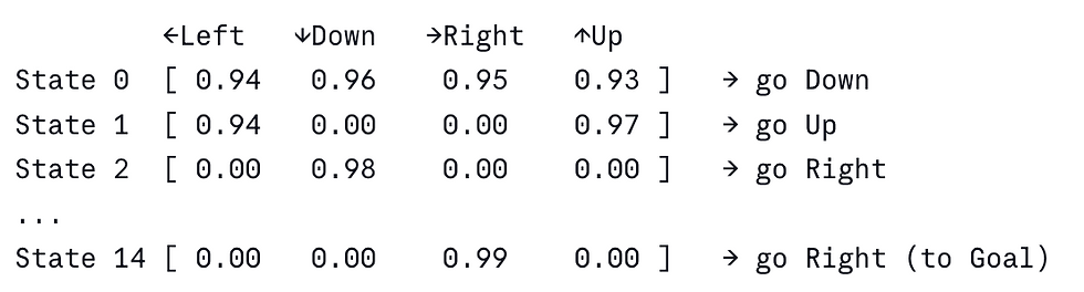
Converged Q-table (selected states):

The agent has learned: "From state 14, go right — that's worth 0.85."

Python Implementation on Frozen Lake


import numpy as np
import gym

# ── Environment ──────────────────────────────────────────
env = gym.make("FrozenLake-v1", is_slippery=False)
n_states  = env.observation_space.n   # 16
n_actions = env.action_space.n        # 4

# ── Hyperparameters ──────────────────────────────────────
EPISODES    = 10_000
ALPHA       = 0.1      # learning rate
GAMMA       = 0.99     # discount factor
EPSILON     = 1.0      # initial exploration rate
EPS_DECAY   = 0.995
EPS_MIN     = 0.01

# ── Q-Table ──────────────────────────────────────────────
Q = np.zeros((n_states, n_actions))

rewards_per_episode = []

# ── Training Loop ─────────────────────────────────────────
for episode in range(EPISODES):
    state, _ = env.reset()
    total_reward = 0
    done = False

    while not done:
        # ε-greedy action selection
        if np.random.random() < EPSILON:
            action = env.action_space.sample()          # explore
        else:
            action = np.argmax(Q[state])                # exploit

        next_state, reward, terminated, truncated, _ = env.step(action)
        done = terminated or truncated

        # Q-Learning update
        td_target = reward + GAMMA * np.max(Q[next_state]) * (not done)
        td_error  = td_target - Q[state, action]
        Q[state, action] += ALPHA * td_error

        state = next_state
        total_reward += reward

    # Decay epsilon
    EPSILON = max(EPS_MIN, EPSILON * EPS_DECAY)
    rewards_per_episode.append(total_reward)

# ── Results ───────────────────────────────────────────────
print(f"Average reward (last 1000 episodes): "
      f"{np.mean(rewards_per_episode[-1000:]):.3f}")

# Visualise learned policy
actions_map = {0: '←', 1: '↓', 2: '→', 3: '↑'}
policy = np.array([actions_map[np.argmax(Q[s])] for s in range(n_states)])
print("\nLearned Policy:")
print(policy.reshape(4, 4))

# ── Output Example ────────────────────────────────────────
# Average reward (last 1000 episodes): 0.974
#
# Learned Policy:
# [['→' '↑' '→' '↑']
#  ['↓' '←' '↓' '←']
#  ['→' '↓' '↓' '←']
#  ['←' '→' '↓' '←']]

Q-Table visualised after training:

Q-Learning vs SARSA vs Monte Carlo

These are the three main families of model-free RL algorithms. Understanding their differences is essential.

Property	Monte Carlo	SARSA (On-Policy TD)	Q-Learning (Off-Policy TD)
Update timing	End of episode	Every step	Every step
Bootstrap?	No	Yes	Yes
Policy type	On-policy	On-policy	Off-policy
What it learns	Value of current policy	Value of current policy	Optimal Q* directly
Bias	Unbiased	Biased	Biased
Variance	High	Low	Low
Handles continuing tasks?	No	Yes	Yes
Risky environments	Neutral	Conservative	Aggressive (optimal)
Convergence	Slow (high variance)	Stable	Fast but can overestimate

Key Difference: Q-Learning vs SARSA

SARSA (on-policy — uses the action actually taken A′):

Q-Learning (off-policy — always uses the best possible next action):

Cliff Walking Example: On a cliff-edge path to the goal, SARSA learns to walk safely away from the cliff (because ε-random steps could fall off). Q-Learning finds the shortest path right along the cliff edge (theoretically optimal but risky with exploration).

The Overestimation Problem

Q-Learning has a systematic upward bias in its Q-value estimates. Here's why.

The TD target is:

If Q(S′,a) contains random noise εa for each action:

Taking the max over noisy estimates always picks the noisily high ones, systematically overestimating.

Illustration:

Double Q-Learning Fix

Use two independent Q networks, Q1Q_1 Q1 and Q2Q_2 Q2:

Standard Q-Learning (same network selects AND evaluates):

Double Q-Learning (Q1 selects, Q2 evaluates):

By decoupling selection from evaluation, the positive bias is broken. Even if Q1 picks a noisily high action, Q2's independent estimate tends to be closer to the true value.

Empirical result: Double DQN reduced value overestimation by 50–90% on Atari games while improving median scores by ~15%.

Deep Q-Networks (DQN)

Tabular Q-Learning fails when state spaces are large or continuous (e.g., 84×84 pixel Atari frames = 33,000+ dimensional input). DQN (Mnih et al., DeepMind 2015) solves this by replacing the Q-table with a neural network.

Architecture

Loss Function

where the TD target uses the frozen target network θ−:

θ = online network weights (updated every gradient step)

θ− = target network weights (frozen for CC C steps, then copied from θ)

Modern Extensions

DQN opened the door to a family of improvements. Here is a roadmap of the major ones:

Convergence and the Deadly Triad

Convergence Guarantees (Tabular)

Q-Learning converges to Q^* if:

All (s,a)(s, a) (s,a) pairs are visited infinitely often
Learning rates satisfy the Robbins-Monro conditions:

Rewards are bounded: ∣R∣ ≤ Rmax⁡
Finite MDP (finite S and A)

The Deadly Triad

With function approximation, convergence guarantees break down. The deadly triad — identified by Sutton & Barto — is the combination of three elements that can cause divergence:

Any two alone are manageable. All three together can cause Q-values to spiral to infinity.

Why DQN works despite this: The experience replay buffer reduces the off-policy problem. The target network slows the bootstrapping instability. Together they tame (but don't eliminate) the deadly triad.

When to Use Q-Learning

Use Q-Learning when:

Action space is discrete and manageable (< ~100 actions)
State space is either small (tabular) or representable by a CNN/MLP (DQN)
You need an off-policy algorithm (want to reuse old experience)
Sample efficiency matters — Q-Learning is more sample-efficient than policy gradient
The task has clear, delayed rewards (Q-Learning handles sparse rewards better than immediate methods)

Conclusion

Q-Learning is, in many ways, the "linear regression" of reinforcement learning — a simple, powerful, well-understood algorithm that serves as the foundation for nearly everything built on top of it.

The key ideas to internalise:

Q(s, a) answers one question: "How much total reward can I expect if I take action a in state s and play optimally from there?"
The Bellman equation gives us a self-consistent definition of Q* — and Q-Learning finds it by resolving prediction errors, one step at a time
The TD error δ is the signal of surprise — positive means better than expected, negative means worse
Q-Learning is off-policy because it always bootstraps toward the best possible future, regardless of exploration
DQN makes Q-Learning scale to complex environments via neural network approximation, experience replay, and target networks
Every major modern RL system — from AlphaGo to robotics controllers — has Q-Learning or its descendants at its core

The algorithm is deceptively simple. Its update rule fits in one line. But the mathematical structure underlying it — Bellman optimality, contraction mappings, the interplay of exploration and exploitation — is deep and rich. Understanding Q-Learning deeply is not just about knowing the algorithm. It is about developing the intuition for how intelligent behaviour can emerge from nothing more than an agent trying to predict its own future.